Cell shading, or fill color, is an effective way to highlight data in a spreadsheet or to indicate that certain cells are associated with one another. But if a cell already has an existing fill color, then you may be looking for a way to change it. Fortunately, cell fill colors can be changed in a manner very similar to how they were set in the first place. You can even choose to remove the fill color of a cell if you wish. Our guide below will show you how to select the cells with the shading that you wish to remove, then direct you to the steps that you need to perform in order to have those cells be filled with a different color.
How to Change the Cell Shading Color in Excel 2010
Our tutorial continues below with additional information on changing the Excel shading color, including pictures of these steps.
How to Change a Fill Color in Excel 2010 (Guide with Pictures)
The steps in this tutorial were written using Microsoft Excel 2010. These steps may vary slightly in different versions of Excel.
Step 1: Open your spreadsheet in Microsoft Excel 2010.
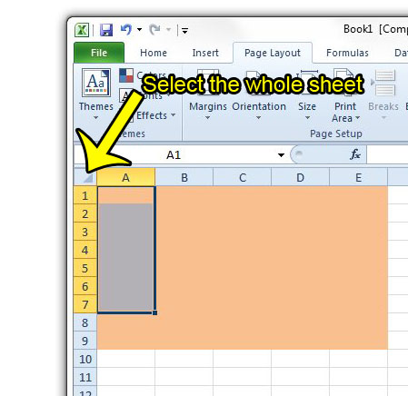
Step 2: Select the cells for which you wish to change the fill color.
Note that you can select an entire row by clicking the row number at the left side of the row, the column by clicking the letter at the top of the column, or the entire sheet by clicking the gray cell above the first row number, and to the left of the first column letter.
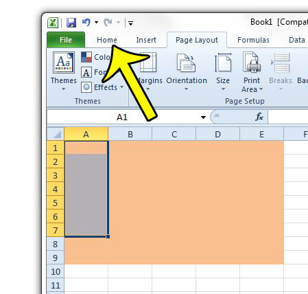
Step 3: Click the Home tab at the top of the window.
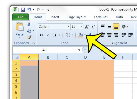
Step 4: Click the down arrow to the right of the Fill Color button.
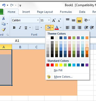
Step 5: Click the color that you wish to use instead.
If you wish to remove the fill color, select the No Fill option. You can continue reading below for additional discussion on changing the Excel fill color.
More Information on How to Use a Different Cell Shading Color in Microsoft Excel
Our guide above has shown you how to select a cell or group of cells that contain a fill color and change it to something else. If you are doing this because the shaded data all shares some type of characteristic, then you may want to explore conditional formatting. This is something that you can use in Microsoft Excel so that it will automatically apply a type of formatting to data if it meets certain criteria. One of these formatting options that you can use involves the fill color. To use conditional formatting you will need to select the data to which you want to apply the formatting, then click the Home tab. You can then click the Conditional Formatting button and make your selection from the options in that drop down menu. If you want to select your entire worksheet then you can click the gray button above the row 1 heading and to the left of the column A heading. You can also press Ctrl + A to select all if you would prefer to use a keyboard shortcut instead. Note that there is a difference between using a white fill color and using no fill color. It may not affect you in many situations, but it can arise if you have something in the background that you need to print, or if you are printing on paper that isn’t white. Are you printing your Excel worksheet, and do you want to make it easier to read? One helpful change to make is to repeat your row of column identifiers at the top of each page. This will make it much easier for people to associate cells with their proper columns and can help to reduce mistakes.
Additional Reading
He specializes in writing content about iPhones, Android devices, Microsoft Office, and many other popular applications and devices. Read his full bio here.