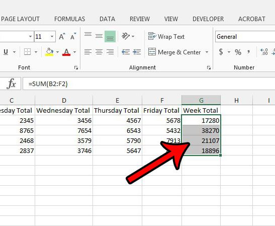
Our guide below will show you how to select a cell or group of cells, then apply formatting that will apply a double underline to the data in those cells. If you are working with a colleague or client that requires certain fields to have double underlines, then you can follow this guide.
How to Double Underline a Value (Numbers or Letters) in Excel 2013
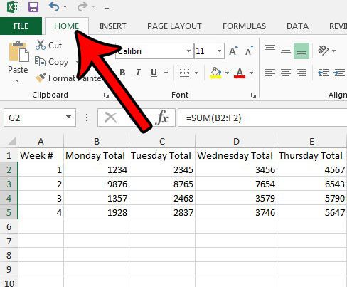
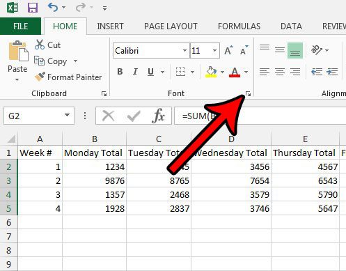
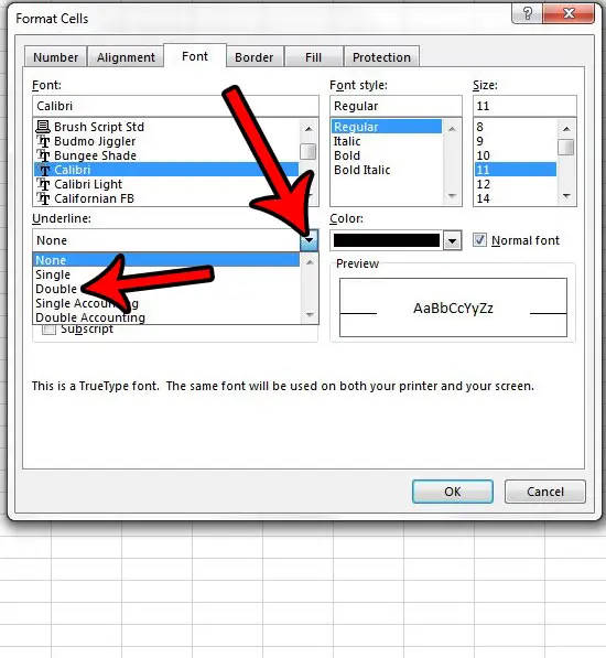
The steps in this article were performed in Excel 2013, but will work in Excel 2010 or 2016 as well. Step 1: Open the spreadsheet containing the value(s) that you wish to double underline. Step 2: Select the cell(s) to which you want to apply the double underline formatting. Note that you can select an entire row by clicking the row number at the left of the sheet, or you can select an entire column by clicking the column letter. Step 2: Click the Home tab at the top of the window. Step 3: Click the small Font Settings button at the bottom-right corner of the Font section of the ribbon. Step 4: Click the Underline dropdown menu, select the Double option, then click the OK button at the bottom of the window. Note that there is also a Double Accounting underline option, if you would prefer to use that styling instead. Is there too much formatting applied to your cells, and it’s becoming difficult to edit or remove it? Learn how to clear all of your cell formatting in Excel and start over with data that doesn’t contain any formatting. After receiving his Bachelor’s and Master’s degrees in Computer Science he spent several years working in IT management for small businesses. However, he now works full time writing content online and creating websites. His main writing topics include iPhones, Microsoft Office, Google Apps, Android, and Photoshop, but he has also written about many other tech topics as well. Read his full bio here.
You may opt out at any time. Read our Privacy Policy


