But that horizontal scroll bar can get in the way if your workbook has a lot of tabs, so you might be looking for a way to hide the scroll bar so that you can see more of your worksheets at once. Our guide below will show you where to find a setting in Excel 2013 that lets you hide the horizontal scroll bar.
How to Stop Showing the Horizontal Scroll Bar in Excel 2013
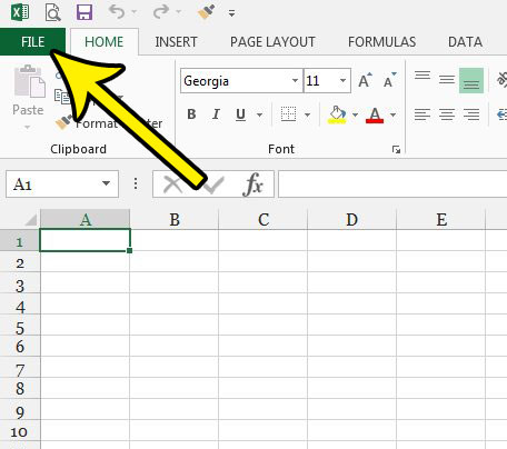
The steps in this article were performed in Microsoft Excel 2013. These steps are going to hide the horizontal scroll bar that appears in the gray bar below the spreadsheet. If you wish to navigate to columns that are to the right or left of what is currently visible on your screen, then you will need to click inside a cell, then move the cursor using the arrow keys on your keyboard. Step 1: Open Excel 2013. Step 2: Choose the File tab at the top-left corner of the window.
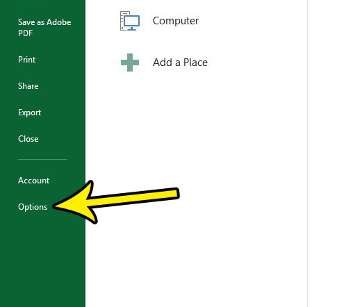
Step 3: Click the Options button at the bottom of the column on the left side of the window.
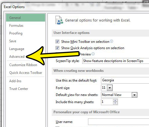
Step 4: Select the Advanced tab at the left side of the Excel Options window.
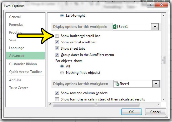
Step 5: Scroll down to the Display options for this workbook section, then click the box to the left of Show horizontal scroll bar to remove the check mark. You can then click the OK button at the bottom of the window.
If you have finally configured your Excel window to look how you want on your screen, then it’s time to start making your printed spreadsheets look right. Read our Excel guide to printing for some tips that can make spreadsheet printing a little easier. He specializes in writing content about iPhones, Android devices, Microsoft Office, and many other popular applications and devices. Read his full bio here.