Learning how to print gridlines in Excel 2013 is a necessity for anyone that often needs to print large spreadsheets. Information in cells can be difficult to read without them, and can lead to mistakes. Data on your screen in Microsoft Excel 2013 is organized efficiently into cells that are separated by gridlines. But when you go to print that spreadsheet, the default setting will not include these gridlines. This results in a sheet with a bunch of data that may seem to run together, or it might be difficult to tell which cell belongs in which row or column. The simplest way to make this document easier to read is by configuring the spreadsheet so that the gridlines are printed. Luckily this is a simple adjustment to make, and the people reading your printed spreadsheets will have an easier time reading them.
How to Print Gridlines in Excel 2013
Our article continues below with additional information on printing gridlines in Excel 2013, including pictures of these steps.
How to Add Gridlines in Excel 2013 (Guide with Pictures)
This is typically one of the first settings I adjust when I am working on a new spreadsheet that I know I will need to print. That way I don’t accidentally print a large spreadsheet without the lines, which can be a waste of paper and time.
Step 1: Open your spreadsheet in Excel 2013.
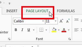
Step 2: Click the Page Layout tab at the top of the window.
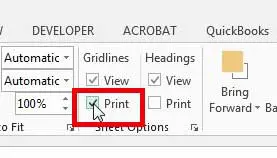
Step 3: Check the box to the left of Print under Gridlines in the Sheet Options section of the ribbon at the top of the window.
This Sheet Options group also includes an option to view gridlines on the screen, as well as options for viewing and printing headers. Now if you press Ctrl + P on your keyboard to open the Print menu, you will see that the gridlines are showing on the spreadsheet in the Print Preview section at the right side of the window. This isn’t the only way to include the gridlines when you are printing a spreadsheet in Excel 2013. Check out the other method below to see if that is something that is easier for you to use.
Alternate method for printing gridlines in Excel
The steps below are longer than the previous method, but will open a Page Setup window where you can center your spreadsheet horizontally or vertically, print the top row on every page, or create and edit a header.
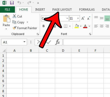
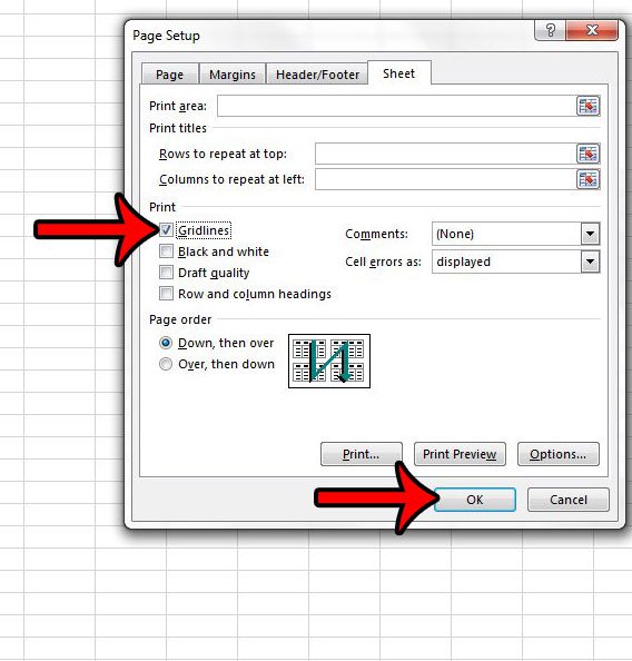
Step 1: Click the Page Layout tab.
Step 2: Click the Page Setup dialog launcher at the bottom-right corner of the Page Setup section in the ribbon.
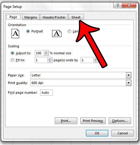
Step 3: Click the Sheet tab at the top of the Page Setup window.
Step 4: Check the box to the left of Gridlines in the Print section of the window. You can click the OK button at the bottom of the window when you are done.
If you have enabled the gridlines to print on your spreadsheet, but you don’t see them, then there may be a fill color applied to those cells. Learn how to remove cell fill color in Excel 2013, then see if your gridlines are printing.
Additional Notes on How to Print the Gridlines in Microsoft Excel
If you only want to print part of your spreadsheet, then you will want to set a Print Area. This option can be found on the Page Layout tab. If you are trying to print a blank spreadsheet full of empty cells, then using a set print area is the way to go.You can navigate to the Print screen to create a print out of your Excel spreadsheet by pressing the Ctrl + P keyboard shortcut. You can also get to the Print menu by clicking the File tab at the top-left of the window and choosing the Print tab from there.Above the Print check box in the Gridlines section of the Sheet Options group is a View option. You can choose that option to hide the gridlines from view on your screen.Cell borders are different from gridlines. You can add or remove cell borders on your Excel sheet by changing the Borders option found on the Home tab.The second method above for printing gridlines in an Excel worksheet involves clicking the Page Setup dialog box on the Page Layout tab, then selecting the Sheet tab. There you will see a Gridlines check box, as well as a handful of other options. These options include printing in draft quality, a drop-down menu to choose whether or not to print comments, and an option to print row or column headings.You can change the format of a cell if you right-click on the cell then choose the Format Cells option. This is helpful if the actual data in your spreadsheet needs to be displayed in a specific format that is different from the current option.Before you click the Print button on the Print menu, be sure to check the Print Preview window to confirm that the gridlines are visible.Opening the Page Setup dialog box can be a more helpful tool when you want to print a spreadsheet and need to change multiple settings for that sheet.If you are trying to print a spreadsheet with gridlines but aren’t planning to put any content in your cells, then you will need to set a print area before you can print that blank spreadsheet. The Print Area option is found on the Page Layout tab in Excel 2013.
If you are printing a multi-page spreadsheet, it is very helpful when you print your column headings on every page, too. Read this article to learn how.
Additional Sources
After receiving his Bachelor’s and Master’s degrees in Computer Science he spent several years working in IT management for small businesses. However, he now works full time writing content online and creating websites. His main writing topics include iPhones, Microsoft Office, Google Apps, Android, and Photoshop, but he has also written about many other tech topics as well. Read his full bio here.
You may opt out at any time. Read our Privacy Policy