I spend a good amount of time working with UPC numbers in Microsoft Excel spreadsheets. One common situation that I encounter is when I have a complete UPC number but need to remove the last digit of the number. This is typically referred to as a check digit and is automatically generated based upon the rest of the numbers in the UPC. While this is a simple task with one or two UPC numbers, it is very tedious when dealing with hundreds or thousands of them. Fortunately, Excel has a formula that will automatically remove the last digit of a number. Simply type the formula into a different cell, and your end result is number minus its last digit. That formula can then be copied down to fill the rest of the cells in a column.
How to Trim the Last Digit Off a Number in Excel 2013
Our tutorial continues below with more on how to remove the last character in Excel, including pictures of these steps. Aside from using formulas to edit data, you can accomplish a lot with formatting options. This convert text to number Excel article will show you how.
How to Remove the Last Digit from a Number in Excel 2013 (Guide with Pictures)
The steps in this article are going to show you how to use a formula to remove the last digit from a number in a cell of your Excel spreadsheet. This means that a cell containing the number “1234” will be trimmed down to “123.” While we will be focusing specifically on removing one digit, you can choose to remove as many digits as you would like by changing the last part of the formula.
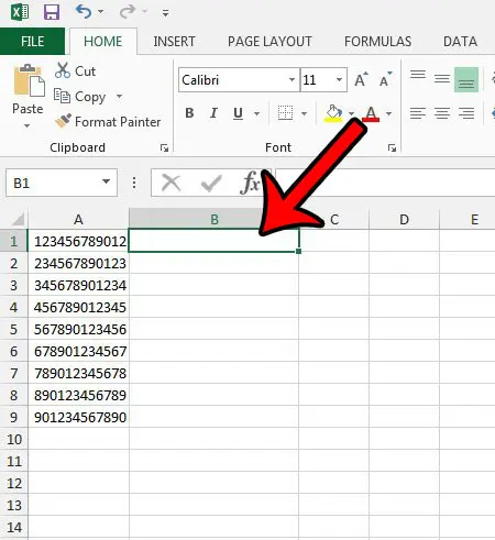
Step 1: Open the spreadsheet containing the cell that you wish to trim.
Step 2: Click inside the cell where you wish to display the number that has had its last digit removed.
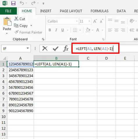
Step 3: Type the formula =LEFT(A1, LEN(A1)-1) into the cell, but replace each A1 with the location of the cell that contains the number for which you want to remove a digit. You can then press Enter on your keyboard to calculate the formula.
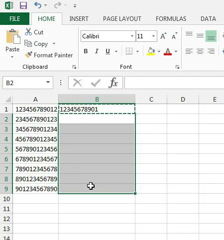
You can then copy the cell containing the formula and paste it into any other cell that contains a number you wish to shorter by one digit. For example, in the image below, I am pasting the formula into cells B2 – B9. Our guide continues below with additional discussion on removing the last digits from numbers in Microsoft Excel. When you have an entire worksheet of data that you don’t need, then our article on deleting Excel sheets will show you how to remove it.
Can I Use the LEN Function to Change the Numeric Value in a Cell?
The section above showed you how to combine the LEN function with the LEFT function to remove the last n characters from a cell, where the “n” value is defined at the end of the formula. We focused specifically on reducing the number of characters in the original value by 1. However, this does more than simply reduce the total length of the value by one or more characters. It also changes the actual value of the data that is displayed in that cell. For example, when you use the LEN function to remove the first or last character from a number or text string it will create a number value or text value that corresponds to this new data set. if you use another user defined function or VBA code to reference the cell where the first character or last character was removed, then that value will be used instead. Basically, this means that the formula doesn’t just produce an empty string or numbers or letters. It is a value that you can use in other formulas. Using the value function (=Value(XX)) will show the current value of that cell, which is the number or text string without the characters from the left side or right side of the original cell’s value. Our Excel #n/a to 0 article can show you a simple way to modify the VLOOKUP formula and make it stop displaying error codes.
More Information on How to Remove Last Digit in Excel 2013
If you wish to shorten a string of characters by more than one digit, then change the number “1” in the formula to the number of digits that you want to remove. For example, if I wanted to remove 4 digits, I would change the formula to =LEFT(A1, LEN(A1)-4). This formula can also be used to remove characters from text strings as well. Tip – If you are also using this formula for UPC reasons, and your number is displaying as scientific notation, then you probably need to change the formatting. This article will show you how to see the formatting applied to a cell, then you can switch to Number or Text formatting instead. The formula that we are using in this article serves the specific purpose of removing characters from the end of a cell’s value. However, this is just one of several related functions that perform similar tasks. For example, there is a MID function that will extract a set of characters from the middle of a cell value. While there is an END function in VBA, it is not a formula that you can type into Excel cells. It also can’t be used to return the “end” characters from a text string.
Additional Sources
After receiving his Bachelor’s and Master’s degrees in Computer Science he spent several years working in IT management for small businesses. However, he now works full time writing content online and creating websites. His main writing topics include iPhones, Microsoft Office, Google Apps, Android, and Photoshop, but he has also written about many other tech topics as well. Read his full bio here.

title: “How To Remove Last Digit In Excel 2013” ShowToc: true date: “2022-12-10” author: “Billie Miller”
I spend a good amount of time working with UPC numbers in Microsoft Excel spreadsheets. One common situation that I encounter is when I have a complete UPC number but need to remove the last digit of the number. This is typically referred to as a check digit and is automatically generated based upon the rest of the numbers in the UPC. While this is a simple task with one or two UPC numbers, it is very tedious when dealing with hundreds or thousands of them. Fortunately, Excel has a formula that will automatically remove the last digit of a number. Simply type the formula into a different cell, and your end result is number minus its last digit. That formula can then be copied down to fill the rest of the cells in a column.
How to Trim the Last Digit Off a Number in Excel 2013
Our tutorial continues below with more on how to remove the last character in Excel, including pictures of these steps. Aside from using formulas to edit data, you can accomplish a lot with formatting options. This convert text to number Excel article will show you how.
How to Remove the Last Digit from a Number in Excel 2013 (Guide with Pictures)
The steps in this article are going to show you how to use a formula to remove the last digit from a number in a cell of your Excel spreadsheet. This means that a cell containing the number “1234” will be trimmed down to “123.” While we will be focusing specifically on removing one digit, you can choose to remove as many digits as you would like by changing the last part of the formula.
Step 1: Open the spreadsheet containing the cell that you wish to trim.
Step 2: Click inside the cell where you wish to display the number that has had its last digit removed.
Step 3: Type the formula =LEFT(A1, LEN(A1)-1) into the cell, but replace each A1 with the location of the cell that contains the number for which you want to remove a digit. You can then press Enter on your keyboard to calculate the formula.
You can then copy the cell containing the formula and paste it into any other cell that contains a number you wish to shorter by one digit. For example, in the image below, I am pasting the formula into cells B2 – B9. Our guide continues below with additional discussion on removing the last digits from numbers in Microsoft Excel. When you have an entire worksheet of data that you don’t need, then our article on deleting Excel sheets will show you how to remove it.
Can I Use the LEN Function to Change the Numeric Value in a Cell?
The section above showed you how to combine the LEN function with the LEFT function to remove the last n characters from a cell, where the “n” value is defined at the end of the formula. We focused specifically on reducing the number of characters in the original value by 1. However, this does more than simply reduce the total length of the value by one or more characters. It also changes the actual value of the data that is displayed in that cell. For example, when you use the LEN function to remove the first or last character from a number or text string it will create a number value or text value that corresponds to this new data set. if you use another user defined function or VBA code to reference the cell where the first character or last character was removed, then that value will be used instead. Basically, this means that the formula doesn’t just produce an empty string or numbers or letters. It is a value that you can use in other formulas. Using the value function (=Value(XX)) will show the current value of that cell, which is the number or text string without the characters from the left side or right side of the original cell’s value. Our Excel #n/a to 0 article can show you a simple way to modify the VLOOKUP formula and make it stop displaying error codes.
More Information on How to Remove Last Digit in Excel 2013
If you wish to shorten a string of characters by more than one digit, then change the number “1” in the formula to the number of digits that you want to remove. For example, if I wanted to remove 4 digits, I would change the formula to =LEFT(A1, LEN(A1)-4). This formula can also be used to remove characters from text strings as well. Tip – If you are also using this formula for UPC reasons, and your number is displaying as scientific notation, then you probably need to change the formatting. This article will show you how to see the formatting applied to a cell, then you can switch to Number or Text formatting instead. The formula that we are using in this article serves the specific purpose of removing characters from the end of a cell’s value. However, this is just one of several related functions that perform similar tasks. For example, there is a MID function that will extract a set of characters from the middle of a cell value. While there is an END function in VBA, it is not a formula that you can type into Excel cells. It also can’t be used to return the “end” characters from a text string.
Additional Sources
After receiving his Bachelor’s and Master’s degrees in Computer Science he spent several years working in IT management for small businesses. However, he now works full time writing content online and creating websites. His main writing topics include iPhones, Microsoft Office, Google Apps, Android, and Photoshop, but he has also written about many other tech topics as well. Read his full bio here.
