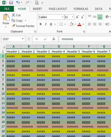
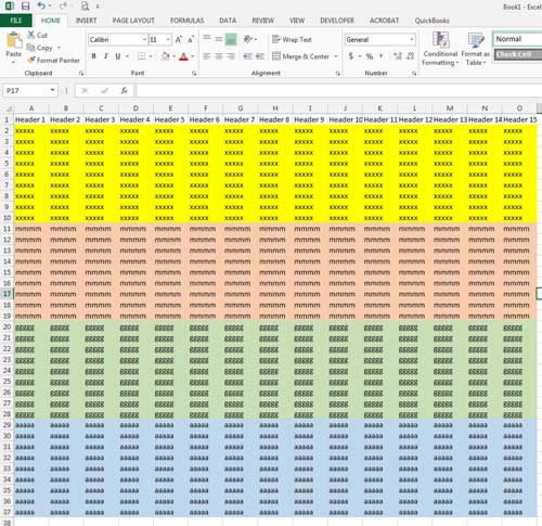
So if you have a spreadsheet that contains rows with fill colors, you can follow our short tutorial below to learn how to sort by color in Excel 2013.
Group Cells by Color in Excel 2013
This tutorial will assume that you have a spreadsheet with rows of cells that have the same fill color. Performing the steps below will group all of the rows with the same color, allowing you to view each group of rows together. Any rows without a fill color will also be grouped together. Step 1: Open your spreadsheet in Excel 2013. Step 2: Select all of the row numbers that you want to sort at the left side of the screen.
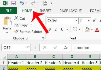
Step 3: Click the Home tab at the top of the window.
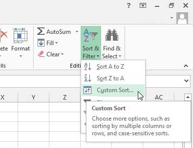
Step 4: Click the Sort & Filter button in the Editing section of the navigational ribbon, then click Custom Sort.
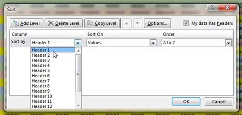
Step 5: Click the drop-down menu next to Sort by, then select the column that you want to use as the sort criteria within the sorted colors.
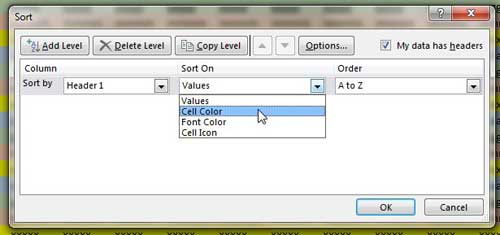
Step 6: Click the drop-down menu under Sort On, then click Cell Color.
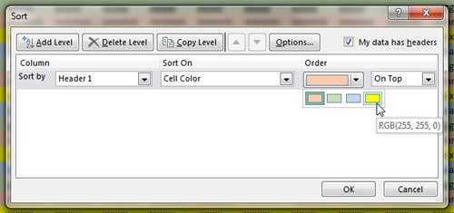
Step 7: Click the drop-down menu under Order, then select the color that you want to be displayed on top.
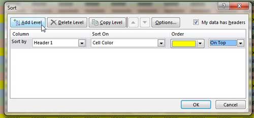
Step 8: Click the Add Level button at the top of the window.
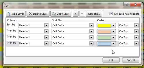
Step 9: Repeat steps 5-8 for the rest of the colors in your spreadsheet.
Step 10: Click the OK button at the bottom of the window when you are done to execute the sort.
Is there too much information in one of your rows, and you want to be able to see all of it? Learn how to expand a row in Excel 2013 and increase your row size. After receiving his Bachelor’s and Master’s degrees in Computer Science he spent several years working in IT management for small businesses. However, he now works full time writing content online and creating websites. His main writing topics include iPhones, Microsoft Office, Google Apps, Android, and Photoshop, but he has also written about many other tech topics as well. Read his full bio here.
You may opt out at any time. Read our Privacy Policy
