Knowing how to hide & unhide columns and rows in Microsoft Excel can give you a lot of options for customizing the data that you display. The benefit of hiding columns versus deleting them is the ability to keep that data in your file so that you can use it later, or if it’s included in a formula. But while hiding a column in Excel is fairly intuitive, trying to unhide columns in Excel can be a little tricky until you learn how it works. Our guide below is going to show you how to go about unhiding hidden columns in an Excel worksheet so that you can view or edit the data contained within that column.
How to Unhide Columns in Excel 2016
Our article continues below with additional information on unhiding columns in Excel, including pictures of these steps.
How to Unhide Hidden Columns in Microsoft Excel 2016, 2019 or Excel for Office 365
The steps in this article were performed in Microsoft Excel for Office 365, but will work in most other versions of Microsoft Excel as well.
Step 1: Open the Excel workbook containing the columns that you would like to unhide.
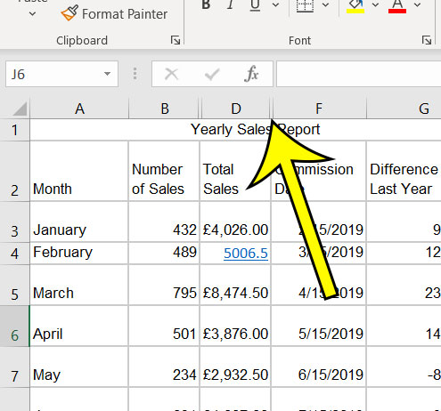
Step 2: Find the hidden columns, as indicated by the two vertical lines identified in the image below.
That double line is a helpful indicator for any hidden columns in your spreadsheet, especially ones that you may have forgotten about or hidden accidentally.
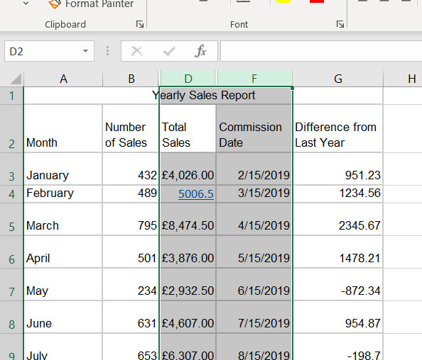
Step 3: Click on the cell to the right of the hidden columns, then keep the mouse held down and drag it to select the column to the left of the hidden columns.
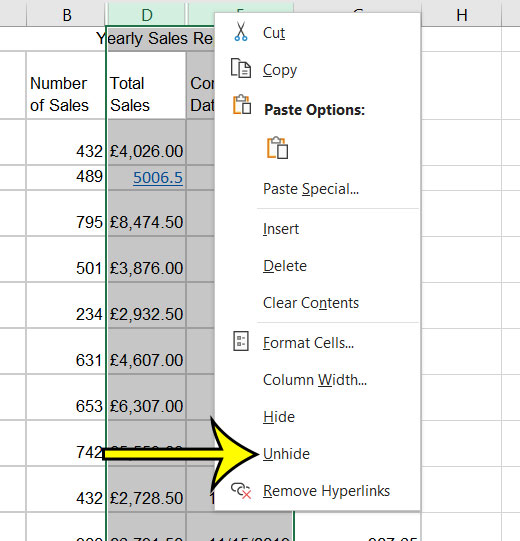
Step 4: Right-click on one of the selected columns, then choose the Unhide option.
Alternate Method for Unhiding Columns in Excel
Aside from the method outlined above, there is another way to unhide columns in Excel. This may be the preferable way to show hidden columns in Excel if you don’t like to right-click, or if you think that you may forget that it’s an option for performing the task.
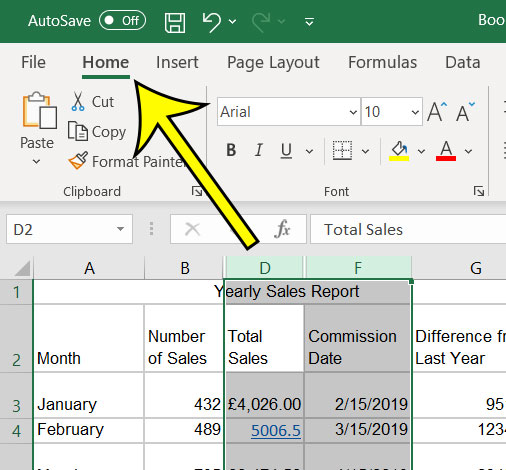
Step 1: Click the Home tab at the top of the window.
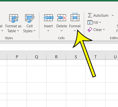
Step 2: Click the Format button in the Cells section at the right side of the ribbon.
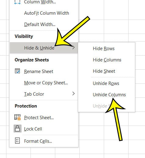
Step 3: Choose the Hide & Unhide option, then click Unhide Columns.
How to Unhide Column A in Excel 2016
Note that there is a special case that comes up if you need to unhide column A. Unhiding the first column in a spreadsheet is a little tricky, as there isn’t a column to the left of it that you can select. Yoou may have even tried to select column B and column C, but unfortunately that doesn’t work either. In order to unhide column A, you are actually going to have to click the button above the row header, and to the left of the column header. This selects the entire spreadsheet. You can then use either of the methods for unhiding columns from the article outlined above. This same information is also applicable if you need to unhide row 1.
Additional Info on Working with Hidden Columns in Microsoft Excel
While the information in this article in concerning with how to unhide columns in Excel, these methods can also be used to unhide hidden rows, too. You will just be looking for two horizontal lines among the row numbers at the left side of the window. You can then use either the right-click method or the Format > Hide & Unhide method to display your hidden rows.You can unhide multiple sections of hidden rows at once in Excel, provided that your column selection is all adjacent columns. If you used the Ctrl key to select multiple non-adjacent columns then the methods for unhiding columns in the sections above will not work.You can select an entire column or an entire row by clicking the corresponding column letter or row number. For example, if I wanted to select all of column A, then I would click the letter “A” in the gray cell above the leftmost column of my spreadsheet.The keyboard shortcut to unhide columns in Excel is Ctrl + Shift + ) . However, this may not work for you, as it didn’t work for me either. Instead you can hold down the Alt key, then press O, followed by C, followed by U. The Alt key needs to be held down as you press each of these keys, and you need to do it relatively fast.The keyboard shortcut to unhide rows is Ctrl + Shift + ( .You can also hide or unhide an entire worksheet in Microsoft Excel as well. This is accomplished by right-clicking on one of the worksheet tabs at the bottom of the window, then choosing the Hide option. If you want to unhide an entire worksheet in Excel, then right-click on a visible worksheet tab, choose the Unhide option, then select the sheet to unhide.While Excel files are able to save all of the formatting changes that you make, other file types may not have that capability. For example, if you have hidden columns in Excel, then save the file as a .csv file, that hidden information will be included and visible in the .csv file.Aside from looking for the double lines to indicate that there are hidden columns, there is also a break in alphabetical order when a column is hidden. This may be a faster way to locate hidden columns if you are having trouble seeing the double lines.
While we briefly covered unhiding an Excel spreadsheet in the section above, you may want to see more about it. This article will give you more information on it, including pictures of the steps.
Additional Reading
He specializes in writing content about iPhones, Android devices, Microsoft Office, and many other popular applications and devices. Read his full bio here.
